Using Random Forest to find important gene markers
- Athena Chu.
- Feb 28, 2019
- 5 min read
It has been a while since my last update, mainly because there are quite a few things to learn before i could implement random forest on the scRNA-seq dataset and interpret the results of the RF model.
Just a few words to capture the minimal concepts and the key terms for understanding random forest.
1) Random forest uses many decision trees for value prediction.
2) Random forest typically bootstraps the data for each decision tree construction – hence generating the in-bag dataset and out-of-bag dataset.
3) The out-of-bag dataset is then used to test the reliability of the constructed trees – hence generating the OOB error rate.
4) Not all predictor variables (aka features) are used for partitioning the dataset at a split in the tree. Usually, a subset of features were randomly selected and the best feauture that partition the dataset would be used in that particular split. The size of the subset of features to consider for each split (mtry) is a parameter we need to optimize.
4.5) How well a feature separating the dataset can be measured by the Gini-impurity. In brief, The Gini-impurity assesses whether the variable of the same class are put to the same side of the tree after the split; if the split put all variable of the same class to one leaf, we achieve the lowest gini-impurity. On the other extreme, if variables of same class were split 50/50 and half of them were put to the left and the other half into the right leaf, the maximum giniimputiry is generated (0.5). More details in K Kong’s post.
Apply random forest to select important gene markers is an attractive approach for scRNA-seq data. One of the scRNA-seq analytuic tools emplolying RF is RAFSIL (Pouyan 2018). Here, i am going to use the standard randomforest package in R instead to get more insights into how the model is derived and if I could retrieve the well characterized cell markers from my random forest model.
This post is inspired by this github page contributed by Braden Katzman & Emily Berghoff (https://github.com/bradenkatzman/CellClassificationMachineLearning). They used scikit to apply several machine learning tactics on the Zeisel 2015 data. We will also use the expression data files provided by the page. But we will use Seurat for the normalisation and then apply Random forrest at the data for classification in R. Then we will use RandomForestExplainer to identify useful gene markers.
First of all, we import and format the expression data file for creating a Seurat object.
‘’’
ann<-read.delim2("expressionmRNAAnnotations.txt", sep="\t", header=F, stringsAsFactors = F)
ann<-ann[1:10, 2:ncol(ann)]
colnames_ann<-as.character(ann[,1])
colnames_ann<-gsub(" ", "_", colnames_ann)
ann<-t(ann)
ann<-ann[2:nrow(ann), ]
base::apply(ann, 2, factor)
colnames(ann)<-as.character(colnames_ann)
ann<-data.frame(ann, stringsAsFactors = F)
row.names(ann)<-ann$cell_id
ann$group_.<-as.numeric(ann$group_.)
ann$total_mRNA_mol<-as.numeric(ann$total_mRNA_mol)
ann$sex<-as.numeric(ann$sex)
ann$age<-as.numeric(ann$age)
ann$diameter<-as.numeric(ann$diameter)
exp<-read.delim2("GSE60361C13005Expression.txt", sep="\t", header=T, stringsAsFactors = F)
exp_rownames<-gsub("-0", "", exp$cell_id)
exp_rownames[10773]<-c("MAR2")
exp_rownames[18089]<-c("MAR1")
rownames(exp)<-exp_rownames
exp<-exp[, 2:ncol(exp)]
colnames(exp)<-ann$cell_id
library(Seurat)
zeisel<-CreateSeuratObject(raw.data=exp, meta.data = ann, project="zeisel2015")
str(zeisel@meta.data)
‘’’
Then, we use Seurat for normalisation and scaling the expression level. We scale the data according to total mRNA content, cell size and tissue of origin.
‘’’
zeisel<-NormalizeData(zeisel)
zeisel<-ScaleData(zeisel, vars.to.regress=c("total_mRNA_mol", "diameter", "tissue"))
‘’’
Next we try to find highly variable genes for the randomforest search
‘’’
zeisel<-FindVariableGenes(zeisel, x.low.cutoff = 1, y.cutoff = 1)
zeisel<-RunPCA(zeisel, pc.genes=zeisel@var.genes, pc.compute=20)
PCAPlot(zeisel)+theme(legend.position = "none")
zeisel<-FindClusters(zeisel, reduction.type = "pca")
zeisel<-RunTSNE(zeisel)
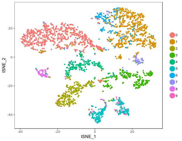
TSNEPlot(zeisel)
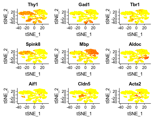
FeaturePlot(zeisel, c("Thy1", "Gad1", "Tbr1", "Spink8", "Mbp", "Aldoc", "Aif1", "Cldn5", "Acta2"))
‘’’
Using the Highly variable genes cut off for expression level of 1 and dispersion of 1, Seurat identified 10 clusters in the data, which is a bit different than the published paper. But the feature plots for the 9 key markers revealed that the clustering is more or less consistent with the published paper.
So now the aim is to filter a batch of informative genes and then run RandomForest to further identify useful features. In this first attempt, I used the highly variable gened identified by Seurat as my input for RF learning, yielding 130 HVG. Unfortunately, Thy1, Tbr1, Spink8, Aif1, Cldn, and Mbp are not in the gene set for RF training as they did not pass the threshold. But I just go ahead.
First I use the tuneRF() function to identify the best mtyr parameter for this gene set (end up being 16). The search began at 11, which is the floored square root of the number of input features; tuneRF tried run a few iteration until the error rate drop no more.
‘’’
library(randomForest)
df<-data.frame(t(zeisel@scale.data[zeisel@var.genes,]), level1class=zeisel@meta.data$level1class)
test_mtyr<-tuneRF(df[, 1:130], df$level1class, stepFactor=1.5, improve=1e-5, ntree=500)
RF_zeisel<-randomForest(level1class ~ ., data = df, mtry=16, localImp = TRUE)
‘’’

Then I run randomForestExplainer to see which are the important genes for the clustering base of minimal tree depth and average gini decrease in the measure_importance() function.
‘’’
library(randomForestExplainer)
min_depth_frame <- min_depth_distribution(RF_zeisel)
head(min_depth_frame, n = 10)
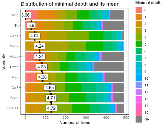
plot_min_depth_distribution(min_depth_frame, mean_sample = "relevant_trees")
importance_frame <- measure_importance(RF_zeisel)
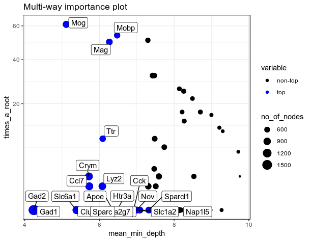
plot_multi_way_importance(importance_frame[importance_frame$gini_decrease>10, ], size_measure = "no_of_nodes", no_of_labels=20)
test_genes<-importance_frame[importance_frame$gini_decrease>20,] %>% arrange(desc(gini_decrease))
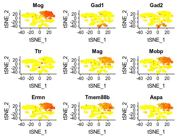
FeaturePlot(zeisel, as.character(test_genes$variable[1:9]))
‘’’
Some of these top 9 most important genes are not previosuly reported by the paper, and intriguingly, they all marking the oligodendrocytes. It is quite similar to the results generated by Seurat FindAllMarkers() function that most marker genes are assign to mark cluster 1 (oligodendrocytes). The overfitting was due to the fact that most cells are oligodendrocytes and pyramidal CA1. Class over representation protentially made the model putting too much effort to distinguish cells belonging/not-belonging to these two class. This will not tell us useful information of gene markers for the other cell types.
Thus, I downsampled the cells according to their level 1 class so that all cell types contain 98 cells (same number as the microglia). I also changed the Seurat FindVariableGenes() cut off to include more genes for the RF model training.
‘’’
zeisel<-FindVariableGenes(zeisel, x.low.cutoff = 0.2, y.cutoff = 0.5)
### 1777 genes now tested , thy1 still not in the pool ###
df<-data.frame(t(zeisel@scale.data[zeisel@var.genes,]), level1class=zeisel@meta.data$level1class)
library(caret)
ddf<-downSample(df, df$level1class)
### downsample to 98 cells per cell type, 686 cells in total ###
### mind that downSample add the category classification in a column to the ddf ##
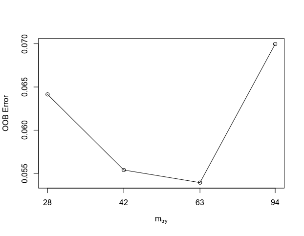
test_mtyr<-tuneRF(ddf[, 1:(ncol(ddf)-2)], ddf$level1class, stepFactor=1.5, improve=1e-5, ntree=500)
### best mtyr=63, increase tree to 1000 ###
RF_zeisel<-randomForest(level1class ~ ., data = ddf[, 1:(ncol(ddf)-1)], mtry=63, localImp = TRUE, ntree=1000)
### OOB error increase by increasing ntree ###
### find important genes again
min_depth_frame <- min_depth_distribution(RF_zeisel)
head(min_depth_frame, n = 10)
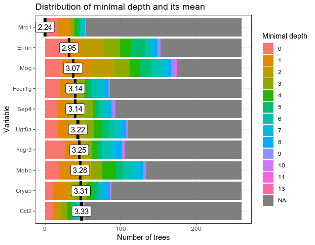
plot_min_depth_distribution(min_depth_frame, mean_sample = "relevant_trees")
min_depth_frame %>% group_by(variable) %>% summarize(rank=mean(minimal_depth)) %>% arrange(rank)
importance_frame <- measure_importance(RF_zeisel)
importance_frame %>% dplyr::filter(variable %in% c("Thy1", "Gad1", "Tbr1", "Spink8", "Mbp", "Aldoc", "Aif1", "Cldn5", "Acta2"))
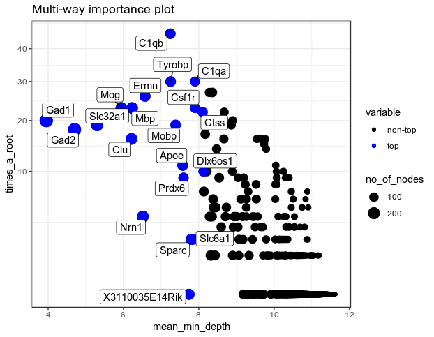
plot_multi_way_importance(importance_frame, size_measure = "no_of_nodes", no_of_labels=20)
test_genes<-importance_frame %>% arrange(desc(gini_decrease))
FeaturePlot(zeisel, as.character(test_genes$variable[1:20]))
‘’’
Ok, with increasing number of features to test, the minimal depth for all the features increase and the gini-decrease deminishes. I think that means we are making bigger trees; and the features are not splitting the variables very well as they encounter different cell types more often, as we have make sure each cell types have the same number of cells in the dataset.
Good news, now I can see more diversity in gene markers highlighting different clusters. The next step is to test the interactions of these important gene markers to build regulatory gene networks, so as to identify the biological relevance of these co-expressed genes as well as better define the cluster to facilitate cell-type characterization.











Comments