On selecting the optimal cluster using SC3
- Athena Chu.
- Jan 18, 2019
- 3 min read
It has been a recurring theme on getting the clustering correct in my quest to learn about ScRNA-seq. In the previous posts I have explored pcaReduce and Seurat (SNN) clustering, in this post I am learning about SC3.
SC3 has been reported to achieve high-accuracy in cluster number inference and it can test a range of cluster parameters for optimization. More specifically, SC3 attains high accuracy through two tactics: Consensus matrix construction and K-means clustering. After normalisation of the count matrix (SC3 suggest log2(m+1) transformation, m=raw count), SC3 constructs a few distant matrices (Euclidean, Pearson, and Spearman as well as their laplacian) and perform PCA on these distance matrix. Next SC3 sample a random number of Pcs to perform k-means clustering with a range of user defined k. Once SC3 has had all the clustering results, it summarizes the results to a consensus matrix from the cell labels. In a particular K-mean clustering result, if two cells are assigned to the same cluster, their similarity is assigned to 1, otherwise 0. SC3 summarizes the pairwise cell-cell similarity by averaging the 1 and 0 across all K-mean clustering results generated from all distant matrices constructed. Then hierarchical clustering is performed on the consensus matrix with a given k-means.
Now comes the key part of determining how many k is optimal! SC3 reports clustering outliers for each k-means and compute Shilhouette for each cluster. I have also read about Dunn test and would like to test it on the SC3 consensus matrices, So lets try it out.
Again, I uses the standard pbmc-2700 dataset provided in the Seurat tutorial. I used Seurat for normalisation and centering. Then I convert the Seurat object to the SingleCellExperiment Object, assigning the raw counts as the raw data and log counts as the normalised data. I only included cells passed the cell-filter and the highly variable genes found by Seurat.
''' R-code
sce <- SingleCellExperiment(
assays = list(
counts = as.matrix(pbmc@raw.data[pbmc@var.genes, colnames(pbmc@data)]),
logcounts = as.matrix(pbmc@data[pbmc@var.genes, ])),
colData = pbmc@meta.data
)
rowData(sce)$feature_symbol <- pbmc@var.genes
sce_sc3 <- sc3(sce, ks = 6:10, biology = TRUE)
'''
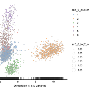
First, I run sc3_estimate_k() on the sclaed data, and it turned out that SC3 estimated the optimal number of cluster is 13. Anyway, I run SC3 with K-mans range of 6 to 10, knowing that the optimal shall be 8 (as shown in Seurat tutorial). When I plotted the PCA using the k-mean = 6 results, I could see that there are already only a few number of cluster outliers. There appears to be limited improvement by increasing the k-mean to 8. So let get more quantitative about our results.
One option is too look at the summarize Silhouette plot. The ideal is that each cell of each cluster achieve a Silhouette index close to 1.
“””
summary<-lapply(sce_sc3@metadata[["sc3"]]$consensus, function(x) as.matrix(x$silhouette)[, c("cluster", "sil_width")])
summary<-lapply(summary, function(x) data.frame(kmeans=max(x[, 1]), cluster=x[, 1], sil_wid=x[, 2]))
summary<-bind_rows(summary)
summary<-summary %>% group_by(kmeans, cluster) %>% summarize(ave=mean(sil_wid))
summary %>% ggplot(aes(x=cluster, y=ave, fill=kmeans, group=kmeans))+
geom_bar(stat="identity", position="dodge")+
scale_x_continuous(breaks=seq(1, 10))
“””
It is quite interesting to see that different cluster respond differently to different k-means. Cluster 1, 5, and 6 reached the highest shilhouette for k-mean equals 7 while cluster 2 and 4 clustered best when k-means equals 10, according to the shilhouette plot.
The next measure is a ad-hoc Dunn test on the consensus matrices. As high similarity in the consensus matrix is close to 1, I transform it back to a distant matrix by 1- consensus. Then we perform Dunn test in R using the Dunn() function. Interestingly, the Dunn index is very small in the transformed consensus matrix and k_mean of 6 actually has the highest Dunn index!

I returned to my pcaReduce hierarchical clustering results and looked at the Dunn index of each of the replicates (100 replicates for 30 to 2 clusters). Again I could see that based on the Pearson correlation matrix, the median Dunn index of having 8 clusters (box plot highlighted in red) is not much better than having 4 to 10 clusters.
‘’’
Output_M <- PCAreduce(t(pbmc_input), nbt=100, q=30, method='M')
library("clValid")
pbmc_dis<-1- cor(pbmc_input, method = "pearson")
### report Dunn test results for each cluster for the whole 100 replicates ###
replicates<-c()
clusters_no<-c()
dunn_index<-c()
for (i in 1:100){
rep_no<-i
replicates<-c(replicates, rep_no)
for (j in 1:ncol(Output_M[[1]])){
clus_no<-max(Output_M[[i]][, j])
clusters_no<-c(clusters_no, clus_no)
dunn_ind<-dunn(distance = pbmc_dis, Output_M[[i]][,j], Data = NULL)
dunn_index<-c(dunn_index, dunn_ind)
}}
peason_cor_dunn<-data.frame(replicates, clusters_no, dunn_index)
peason_cor_dunn%>%
ggplot(aes(y=dunn_index, x=clusters_no, colour=replicates, group=clusters_no))+
geom_boxplot()+
geom_boxplot(data=subset(peason_cor_dunn, clusters_no==8), fill="red")
‘’’

So maybe in the end of the days, focusing of which markers are under differential expression would help to group cells effectively into clusters. But it will post a challenge if the defferential expression of these markers are gradual and operate in conchord with other markers. This is typical in cell differentiation that the cell identity is determined by a combined effects of various transcription factor gradients. In these cases, setting a threshold in a gradient of marker gene expression or even a combination of gradients will be the key issue of refining sub-populations in the single-cell experiments.


Comments